TI-BASIC:Tcdf: Difference between revisions
Initial automated import |
KermMartian (talk | contribs) No edit summary |
||
| Line 21: | Line 21: | ||
Alternatively, you can exploit the identity | Alternatively, you can exploit the identity | ||
<math> | |||
\operatorname{tcdf}(-\infty,0,\nu)=\frac1{2} | \operatorname{tcdf}(-\infty,0,\nu)=\frac1{2} | ||
</math> | |||
(similarly for the interval from 0 to ∞) | (similarly for the interval from 0 to ∞) | ||
| Line 29: | Line 29: | ||
and thus | and thus | ||
<math> | |||
\operatorname{tcdf}(-\infty,x,\nu)=\frac1{2}+\operatorname{tcdf}(0,x,\nu) | \operatorname{tcdf}(-\infty,x,\nu)=\frac1{2}+\operatorname{tcdf}(0,x,\nu) | ||
</math> | |||
For the form used in two-tailed tests, the following identity may be useful: | For the form used in two-tailed tests, the following identity may be useful: | ||
<math> | |||
\operatorname{tcdf}(-x,x,\nu)=2\operatorname{tcdf}(0,x,\nu) | \operatorname{tcdf}(-x,x,\nu)=2\operatorname{tcdf}(0,x,\nu) | ||
</math> | |||
= Formulas = | = Formulas = | ||
| Line 43: | Line 43: | ||
As with any other continuous distribution, tcdf( can be defined in terms of the probability density function, [[TI-BASIC:Tpdf|Tpdf(]]: | As with any other continuous distribution, tcdf( can be defined in terms of the probability density function, [[TI-BASIC:Tpdf|Tpdf(]]: | ||
<math> | |||
\operatorname{tcdf}(a,b,\nu)=\int_a^b \operatorname{tpdf}(t,\nu)\mathrm{d}t | \operatorname{tcdf}(a,b,\nu)=\int_a^b \operatorname{tpdf}(t,\nu)\mathrm{d}t | ||
</math> | |||
The function can also be expressed in terms of an [http://mathworld.wolfram.com/IncompleteBetaFunction.html incomplete beta function]. | The function can also be expressed in terms of an [http://mathworld.wolfram.com/IncompleteBetaFunction.html incomplete beta function]. | ||
| Line 51: | Line 51: | ||
For one degree of freedom (ν=1), tcdf( is expressible in terms of simpler functions: | For one degree of freedom (ν=1), tcdf( is expressible in terms of simpler functions: | ||
<math> | |||
\operatorname{tcdf}(a,b,1)=\frac1{\pi}\left(\tan^{-1}\left(b\right)-\tan^{-1}\left(a\right)\right) | \operatorname{tcdf}(a,b,1)=\frac1{\pi}\left(\tan^{-1}\left(b\right)-\tan^{-1}\left(a\right)\right) | ||
</math> | |||
This is the so-called Cauchy distribution. | This is the so-called Cauchy distribution. | ||
Latest revision as of 19:24, 24 February 2016
Command Summary
Calculates the Student's t probability betwen lower and upper for degrees of freedom ν.
Command Syntax
tcdf(lower, upper, ν)
Menu Location
Press:
- 2ND DISTR to access the distribution menu
- 5 to select tcdf(, or use arrows.
Press 6 instead of 5 on a TI-84+/SE with OS 2.30 or higher.
TI-83/84/+/SE
2 bytes
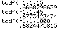
tcdf( is the Student's t cumulative density function. If some random variable follows this distribution, you can use this command to find the probability that this variable will fall in the interval you supply.
Unlike Normalcdf(, this command only works for the standardized distribution with mean 0 and standard deviation 1. To use it for non-standardized values you will have to standardize them by calculating (X-μ)/σ (where μ is the mean and σ the standard deviation). Do this for both lower and upper.
Advanced
Often, you want to find a "tail probability" - a special case for which the interval has no lower or no upper bound (the form frequently used in one-tailed tests). For example, "what is the probability x is greater than 2?". The TI-83+ has no special symbol for infinity, but you can use E99 to get a very large number that will work equally well in this case (E is the decimal exponent obtained by pressing [2nd] [EE]). Use E99 for +∞, and -E99 for -∞.
Alternatively, you can exploit the identity
<math> \operatorname{tcdf}(-\infty,0,\nu)=\frac1{2} </math>
(similarly for the interval from 0 to ∞)
and thus
<math> \operatorname{tcdf}(-\infty,x,\nu)=\frac1{2}+\operatorname{tcdf}(0,x,\nu) </math>
For the form used in two-tailed tests, the following identity may be useful:
<math> \operatorname{tcdf}(-x,x,\nu)=2\operatorname{tcdf}(0,x,\nu) </math>
Formulas
As with any other continuous distribution, tcdf( can be defined in terms of the probability density function, Tpdf(:
<math> \operatorname{tcdf}(a,b,\nu)=\int_a^b \operatorname{tpdf}(t,\nu)\mathrm{d}t </math>
The function can also be expressed in terms of an incomplete beta function.
For one degree of freedom (ν=1), tcdf( is expressible in terms of simpler functions:
<math> \operatorname{tcdf}(a,b,1)=\frac1{\pi}\left(\tan^{-1}\left(b\right)-\tan^{-1}\left(a\right)\right) </math>
This is the so-called Cauchy distribution.
